
Exploring One-Variable Data Practice Test
Question
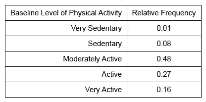
Arthur is the manager of a recently opened 24-hour gym. He wanted to know the baseline level of physical activity (PA) of new gym enrollees and decided to include a small survey in the enrollment application during a certain month. The survey asked individuals to rate their baseline level of PA as very sedentary, sedentary, moderately active, active, or very active. The relative frequency of each baseline level of PA of new enrollees who completed the survey is shown in the table below.
Which of the following statements must be true?
| A. Fewer new enrollees reported an active or very active rather than a moderately active baseline level of PA. | |
| B. More than half of the new enrollees reported having a moderately active baseline level of PA. | |
| C. Out of all new enrollees who completed the survey, 10 reported having a sedentary baseline level of PA. | |
| D. The number of new enrollees who reported having a very sedentary or sedentary baseline level of PA is 12. | |
| E. The proportion of new enrollees who reported having an active baseline level of PA is 0.91. |
Hint:
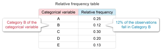
A relative frequency table gives the proportion of observations that fall into each category of a categorical variable.
Explanation
A relative frequency table gives the proportion of observations that fall into each category of a categorical variable.
The table of physical activity (PA) shows the proportion of the baseline levels of PA of new gym enrollees. Eliminate Choices C and D because the total number of enrollees is unknown and cannot be determined from the information given.
Notice that the proportion of new enrollees reporting a moderately active baseline PA level is 0.48 and that the proportion reporting an active or very active baseline PA level is 0.27 + 0.16 = 0.43.
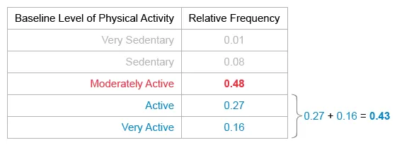
This finding means that the proportion of new enrollees reporting an active or very active baseline PA level (0.43) is less than the proportion reporting a moderately active baseline PA level (0.48).
Therefore, the statement that must be true is:
| Fewer new enrollees reported an active or very active rather than a moderately active baseline level of PA. |
(Choice B) The proportion of new enrollees who reported having a moderately active baseline level of PA (0.48) is less (not more) than half (0.50).
(Choices C and D) It is not possible to determine the number of new enrollees reporting each baseline level of PA because no information is given about the total number of new enrollees surveyed.
(Choice E) The proportion of new enrollees who reported having an active baseline level of PA is 0.27 (not 0.91). The value 0.91 is the proportion of new enrollees who reported having a moderately active, active, or very active baseline level of PA (0.48 + 0.27 + 0.16 = 0.91).
Things to remember:
A relative frequency table gives the proportion of observations that fall into each category of a categorical variable.
Question
The frequency distribution of students by class in a random sample of 50 students in a particular academic year at a local college is shown in the table below.

The Office of Academic Affairs decides to reclassify students. It will now group freshmen and sophomores together as underclassmen and group juniors and seniors together as upperclassmen. Which of the following represents the relative frequency distribution of students for the new classification?
A.  |
|
B.  |
|
C.  |
|
D.
|
|
E. 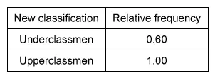
|
Hint:
A frequency table gives the number of observations for each category of a categorical variable.
A relative frequency table gives the proportion of observations for each category.
Explanation
A frequency table gives the number of observations that fall into each category of a categorical variable.
A relative frequency table gives the proportion of observations that fall into each category.
A proportion in fraction form represents a part (numerator) of a whole (denominator):
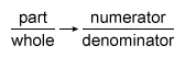
It is possible to calculate the entire relative frequency table, but notice that all the choices have a different value for upperclassmen. Calculate the proportion of upperclassmen in the sample.
The whole (denominator) is the total number of students in the sample.
The part (numerator) is the number of upperclassmen.

The number of students in the sample is 50, so the whole is 50.
To find the part, add together the number of juniors and seniors (upperclassmen).
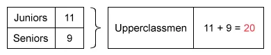
To calculate the proportion of upperclassmen, divide the number of upperclassmen (part) by 50 (whole).

Among the choices, only Choice B shows a relative frequency table with a proportion of 0.40 for upperclassmen.
(Choice A) This table may result from mistakenly dividing the observed distribution in each class by 100, rather than by the total number of students in the sample (50).
(Choice C) This table represents a relative distribution where all classes have the same frequency of students, but the classes do not have the same frequency.
(Choice D) This table may result from mistakenly switching the frequencies of underclassmen and upperclassmen when creating the new classification table.
(Choice E) This table represents the cumulative distribution, not the relative distribution.
Things to remember:
- A frequency table gives the number of observations that fall into each category of a categorical variable.
- A relative frequency table gives the proportion of observations that fall into each category.
Question
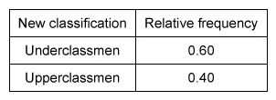
A teacher asked the 20 students in a classroom which season of the year they liked the most. The results of the survey are shown in the relative frequency table below. Notice that the information about students who liked fall the most is missing.
Which of the following is the frequency of students who liked fall the most?
| A. 8 | |
| B. 10 | |
| C. 12 | |
| D. 20 | |
| D. 40 |
Explanation
The relative frequencies must add up to 1, so the relative frequency of students who liked fall is 1 − 0.20 − 0.25 − 0.15 = 0.40. Multiply this relative frequency by the total number of students in the classroom to find the frequency: 0.40 × 20 = 8.
Exploring Two-Variable Data Practice Test
Question
Candy companies X, Y, and Z make boxes of gummies in five fruit flavors. Anna bought a box from each company and determined the number of gummies of each flavor. The graph below shows the relative frequency distribution of flavors for each box of gummies.
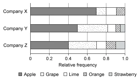
Which of the following statements must be true?
| A. The number of lime gummies in the Company X box was equal to the sum of the number of lime gummies in the other two boxes. | |
| B. There were fewer grape gummies in the Company X box than in the Company Y box. | |
| C. There were more apple gummies than grape gummies in the Company Y box. | |
| D. There were more grape gummies than apple gummies in the Company Z box. | |
| E. There was the same number of lime gummies in the Company Y box as in the Company Z box. |
Hint:
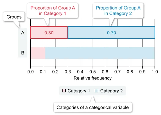
The width (or height) of segments in a segmented bar graph indicates either the relative frequency or counts of each category of a categorical variable.
Explanation
Each bar in a segmented bar graph represents a single group, and the width (or height) of the segments within each bar represents either the relative frequency or count of each category of a categorical variable in that group.
Note: A segmented bar graph of relative frequencies does not allow for a comparison of the number of observations per segment between groups unless the total number of observations in each group is given.
Analyze each answer choice to determine which of the statements is true, and recall that it is possible to compare only within the same box (because the total numbers of gummies in the boxes are not given).
Notice that in the Company Y box, the segment for apple gummies is larger than the segment for grape gummies.
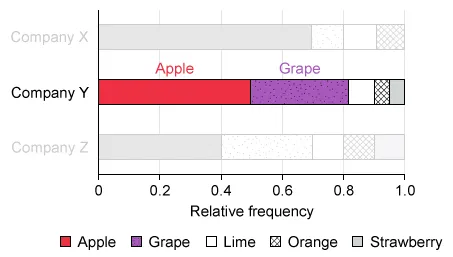
The relative frequency of apple gummies in the Company Y box is greater than grape gummies because the segment for apple gummies is longer than the segment for grape gummies (0.50 > 0.32).
Therefore, there were more apple gummies than grape gummies in the Company Y box.
(Choices A, B, and E) These statements are not true because the total number of gummies in each box is unknown and the given chart shows only relative frequencies (proportions). Therefore, it is impossible to compare the number of gummies of each flavor in different company boxes.
(Choice D) This statement is not true because the relative frequency of grape gummies in the Company Z box is approximately 0.3 and the relative frequency of apple gummies is 0.4.
Things to remember:
-
A segmented bar graph displays either the relative frequency or count distribution of a categorical variable in each of several groups.
-
A segmented bar graph of relative frequencies does not allow for a comparison of the number of observations per segment between groups unless the total number of observations in each group is given.
Question
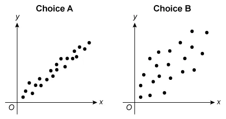
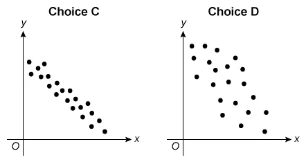
For which of the following scatterplots is the correlation between x and y closest to 0 ?
A. 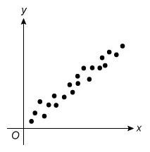 |
|
B. 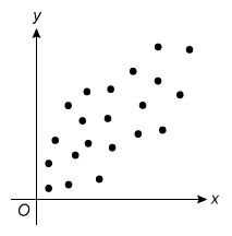 |
|
C. 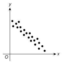 |
|
D.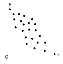
|
|
E. 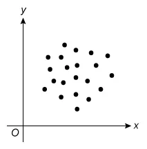
|
Hint:
The correlation coefficient describes the direction and strength of the relationship between two variables x and y.
Explanation
The correlation coefficient r describes the direction and strength of a linear relationship between two quantitative variables x and y. The magnitude of r indicates the strength of the relationship, and the sign of r indicates the direction.
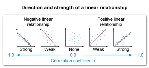
The question asks which scatterplot has a correlation closest to 0 (r = 0), which describes data with no linear relationship. Eliminate Choices A, B, C, and D because they show a linear relationship.
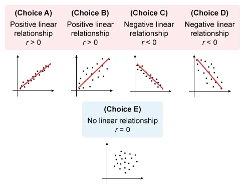
Of the choices, the scatterplot for which the correlation between x and y is closest to 0 is Choice E.
(Choices A and B)These scatterplots show different levels of strength of positive linear relationships (r > 0). However, the question asks for the plot with a correlation closest to 0 (r = 0).
(Choices C and D)These scatterplots show different levels of strength of negative linear relationships (r < 0). However, the question asks for the plot with a correlation closest to 0 (r = 0).
Things to remember:
- The correlation coefficient r describes the direction and strength of the relationship between two variables x and y.
- When two variables x and y do not show a linear relationship, the correlation coefficient r is equal to or close to 0.
Question
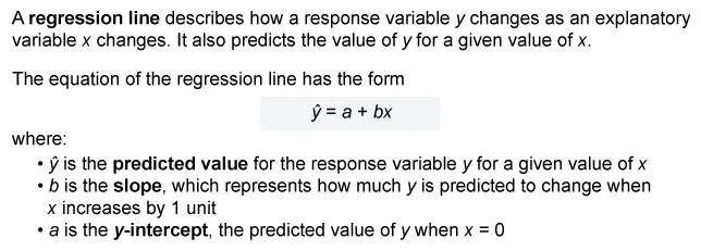
A pediatrician collected data on the age (in months) and length (in inches) of a random sample of boys between the ages of 1 and 12 months. A scatterplot of the data showed a strong linear relationship. The following regression was created:
length = 21.113 + 0.641(months)
The pediatrician uses the regression equation to predict the length of a 9-month-old boy and of an 18-month-old boy. Which of the following is a possible reason why the predicted length of the 9-month-old boy is more reliable than the predicted length of the 18-month-old boy?
| A. An age of 18 months is outside the interval of ages used to generate the regression equation. | |
| B. The age may not explain much of the variation in length. | |
| C. The correlation coefficient is positive. | |
| D. The slope of the sample regression line is greater than 0. | |
| D. The y-intercept of the sample regression is positive. |
Hint:
Extrapolation is the prediction of a response value for a value for the explanatory variable that is outside the interval of values used to determine the regression line.
Explanation
Extrapolation is the prediction of the value of the response variable y for a value for the explanatory variable x that is outside the interval of the x-values used to determine the regression line.
The predicted value is less reliable the further outside the x-values used to determine the regression line.
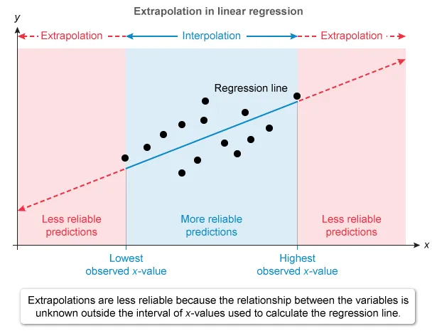
The regression predicts length (y) from the age (x) of boys aged 1 to 12 months, so the observed x-values range from 1 to 12 months. Unlike for a 9-month-old boy, the prediction for an 18-month-old is an extrapolation.
Therefore, the reason why the predicted length of the 9-month-old boy is more reliable than the predicted length of the 18-month-old boy is:
| An age of 18 months is outside the interval of ages used to generate the regression equation. |
(Choice B) The amount of variation in length explained by age describes how well the regression line fits the data, but it does not help to explain why a predicted value would be more precise than another.
(Choice C) A positive correlation coefficient indicates that as age increases, length tends to increase, but it does not help to explain why a predicted value would be more precise than another.
(Choices D and E) The slope and the y-intercept describe the regression line used to predict the length of boys from their age, but it does not help to explain why a predicted value would be more precise than another.
Things to remember:
-
Extrapolation is the prediction of the value of the response variable y for a value for the explanatory variable x that is outside the interval of x-values used to determine the regression line.
-
The predicted value is less reliable as an estimate the further the extrapolation.
Collecting Data Practice Test
Question
An investigator conducted a study to determine the effects of a new hair-growth shampoo for women with thinning hair. A total of 50 women with thinning hair volunteered to participate in the study. The women were randomly assigned to either the new shampoo or regular shampoo. At the end of a 12-week period, the change in hair length for each woman was recorded. The women in the group using the new shampoo had, on average, a greater change in hair length than the women in the group using regular shampoo. Which of the following is the most appropriate conclusion?
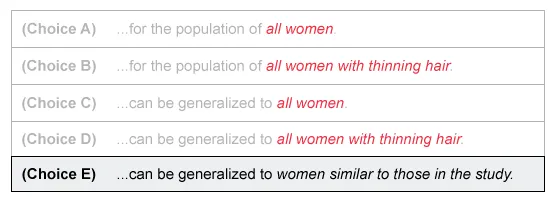
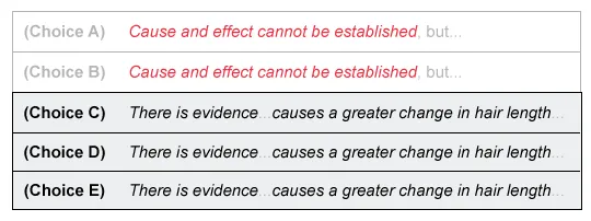
| A. Cause and effect cannot be established, but there is an association between using the new shampoo and a greater change in hair length for the population of all women. | |
| B. Cause and effect cannot be established, but there is an association between using the new shampoo and a greater change in hair length for the population of all women with thinning hair. | |
| C. There is evidence that using the new shampoo causes a greater change in hair length than using regular shampoo, and the conclusion can be generalized to all women. | |
| D. There is evidence that using the new shampoo causes a greater change in hair length than using regular shampoo, and the conclusion can be generalized to all women with thinning hair. | |
| E. There is evidence that using the new shampoo causes a greater change in hair length than using regular shampoo, and the conclusion can be generalized to women similar to those in the study. |
Hint:
To generalize results to a population, study participants must be randomly selected from that population.
To establish a cause-and-effect relationship, study participants must be randomly assigned to treatments.
Explanation
In statistical inference, the purpose is to make inferences about a population or about cause-and-effect relationships.
To generalize results to a population, study participants must be randomly selected from that population.
To establish a cause-and-effect relationship, study participants must be randomly assigned to treatments.
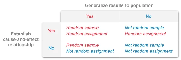
Determine whether results generalize to a larger population (random sample) and whether it is possible to establish a cause-and-effect relationship (random assignment).
Note: If the sample was randomly selected, identify the population from which it was chosen.
Generalize results to a population:
It is given that women volunteered to participate in the study, so women were not randomly selected, and results do not generalize to any other population of women not similar to those in the study.
It is possible to eliminate Choices A, B, C, and D because they generalize to populations larger than women in the study (all women and all women with thinning hair).
Establish a cause-and-effect relationship:
It is given that women were randomly assigned to shampoos (treatments), so the results of the study are evidence of cause and effect between the type of shampoo and change in hair length.
It is possible to eliminate Choices A and B because they state that cause and effect cannot be established.
By a process of elimination, there is evidence that using the new shampoo causes a greater change in hair length than using regular shampoo, and the conclusion can be generalized to women similar to those in the study.
Things to remember:
-
If study participants are randomly chosen, results generalize to the population from where they were selected. Otherwise, results generalize to the sample under study and similar individuals.
-
If study participants are randomly assigned to treatments, results are evidence of a cause-and-effect relationship. Otherwise, results are evidence of statistical association.
Question
A psychologist is interested in the development of figure-ground color perception in infants. She randomly selected 6 five-month-old infants, 6 seven-month-old infants, 6 nine-month-old infants, and 6 eleven-month-old infants. The psychologist then measured the ability of the infants to detect colored objects on checkered backgrounds. Which of the following best describes the psychologist's sampling method?
| A. A cluster random sample | |
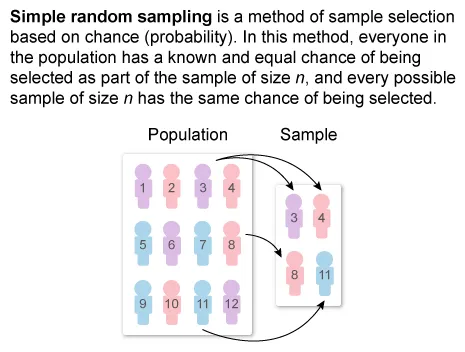
| B. A simple random sample | |
| C. A stratified random sample | |
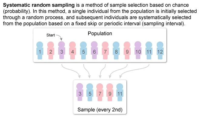
| D.A systematic random sample | |
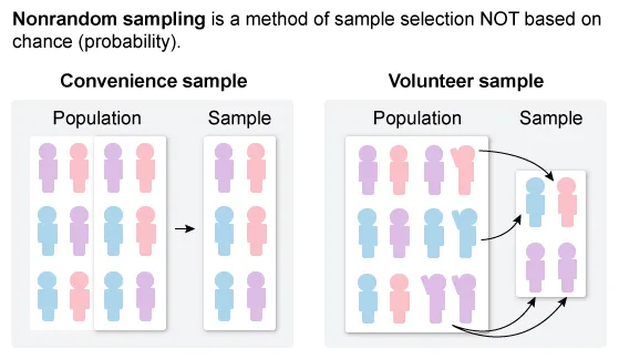
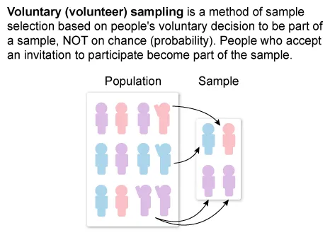
| E. A volunteer sample |
Hint:
To identify the sampling method in a study, evaluate whether random selection is used and whether individuals are selected directly from the population or from groups within the population.
Explanation
To identify the sampling method in a study, determine whether the selection of individuals is random or nonrandom, and if individuals are selected from directly from a population or from groups within a population.
It is given that the psychologist randomly selected infants from 4 groups of infants of different ages, so the population was divided by age and then independent random samples were taken from each age group.
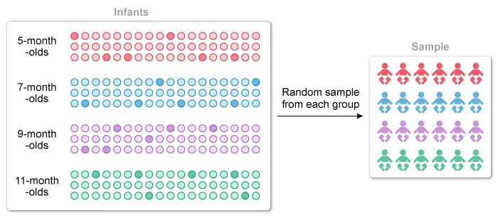
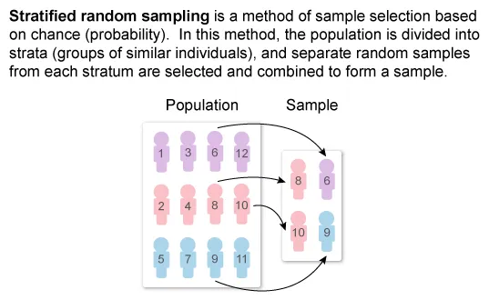
This method of sampling is known as stratified random sampling, where the population is divided into groups (strata) and independent random samples from each group (stratum) are selected and combined to form a sample.
Therefore, the psychologist's sampling method is best described as a stratified random sample.
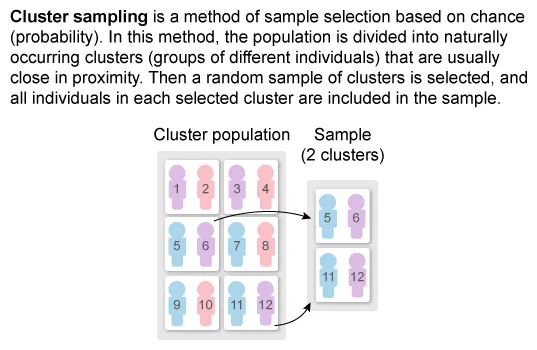
(Choice A) In a cluster random sample, the population is divided into smaller similar groups (clusters), and data from all individuals in randomly selected clusters are used. However, the psychologist randomly selected children within every age group (strata), rather than selecting all individuals in a sample of groups.
(Choice B) For a simple random sample, individuals are selected directly from the population to form the sample. However, the psychologist did not randomly select 24 infants from the population of infants, but instead randomly selected six infants from each of the four age groups (strata).
(Choice D) In a systematic random sample, a random member from the population is selected and subsequent individuals are selected based on fixed or periodic intervals.
(Choice E) A volunteer sample is an example of nonrandom sampling methods. However, the psychologist used a random sampling method.
Things to remember:
In stratified random sampling, the population of interest is divided into different strata based on a common characteristic, and a simple random sample is then chosen from each stratum and combined to form a sample.
Question
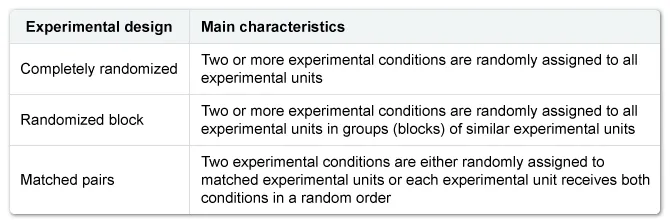
A researcher wants to conduct a study to compare the effect of using nicotine patches, nicotine gums, and a multi-faceted approach that may include counseling, support groups, and behavioral therapy to help adults quit smoking. He is concerned that the effects of these approaches vary depending on the number of packs of cigarettes smoked per day. Which of the following research designs would be most appropriate to address the researcher's concern?
| A. A completely randomized design | |
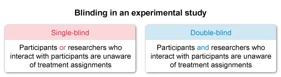
| B. A double-blind experimental design | |
| C. A matched-pairs design | |
| D. A single-blind experimental design | |
| E. A randomized complete block design |
Hint:
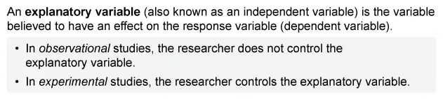
Consider that there are three variables of interest: the treatments, the response, and a third variable that the researcher is concerned about.
Explanation
It is given that a researcher is concerned that the effect of three nicotine treatments (patches, gums, and multi-faceted approach) on quitting smoking varies depending on the number of packs of cigarettes smoked per day.
There are three variables of interest: the three treatments, the response, and a third variable that the researcher is concerned about.

Consider that blinding helps prevent bias but will not help control for differences in the effect of the nicotine treatments based on the number of packs of cigarettes smoked. Eliminate Choices B and D.
To determine which research design would be most appropriate to address the researcher's concern, consider how many variables are accounted for in each of the most common experimental designs.
Notice that the study compares three treatments, so eliminate Choice C.
To account for the effect the number of packs of cigarettes smoked per day has on the treatments, it is necessary to group subjects based on number of packs smoked per day and then evaluate each group separately.
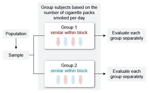
This research design would control how the effects of the treatments vary depending on the number of packs of cigarettes smoked per day.
Therefore, the research design that would be most appropriate to address the researcher's concern is the randomized complete block design.
(Choice A) A completely randomized design can compare the effect of the treatments on the response (quitting smoking), but will not account for the number of cigarettes smoked per day (the researcher's concern).
(Choices B and D) Blinding controls bias but does not help evaluate the effect of different treatments.
(Choice C) A matched-pairs design can help control for differences in the effect of the treatments due to the number of packs of cigarettes smoked per day if there are two treatments. However, the study has three treatments.
Things to remember:
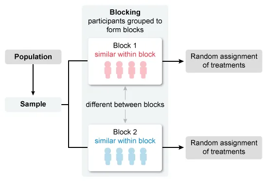
A randomized complete block design allows the evaluation of treatment effects in groups (blocks) of similar individuals (experimental units). It is the most appropriate design when the effect of treatments varies based on another variable.
Probability, Random Variables and Probability Distributions Practice Test
Question
In a simulated game, the roll of a fair six-sided die is randomized according to a computer. The computer software was written to guarantee that rolls are independent and that the probability of the number 2 landing faceup is equal to . If the computer software is functioning correctly, which of the following statements must be true?
-
In repeated simulations, the relative frequency with which the number 2 will land faceup in the long run is equal to .
-
If after several repetitions the relative frequency of the number 2 landing faceup is less than , then the probability that the number 2 lands faceup will increase for future simulations.
-
The relative frequency will equal the probability if the number of simulations is greater than 30.
| A. I only | |
| B. II only | |
| C. I and II only | |
| D. I and III only | |
| E. I, II, and III |
Hint:
Probability is the relative frequency of an outcome of a chance process in the long run.
Explanation
A probability is the relative frequency of an outcome of a chance process when the process is repeated many times (long-run frequency).
The law of large numbers states that as the number of independent trials of a chance process increases, the observed relative frequency of an outcome gets closer to its expected relative frequency (probability).
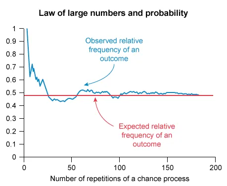
When the number of trials is small, the relative frequency may differ from the true expected relative frequency due to random variation. Determine whether each statement is true.
Statement I: In repeated simulations, the relative frequency with which the number 2 will land faceup in the long run is equal to .
If the computer software is functioning correctly, the probability that the number on the fair six-sided die that lands faceup is 2 is equal to .
This statement is true because the law of large numbers guarantees that the probability of an event is equal to the expected long-run frequency of that event. It is possible to eliminate Choice B.
Statement II: If after several repetitions the relative frequency of the number 2 landing faceup is less than , then the probability that the number 2 lands faceup will increase for future simulations.
If the computer software is functioning correctly, then the simulated rolls are independent. Events are independent if the occurrence of one event does not impact the probability of the other.
This statement is false because the probability (likelihood) that the number 2 lands faceup is not impacted by earlier rolls of the die. It is possible to eliminate Choices B, C, and E.
Statement III: The relative frequency will equal the probability if the number of simulations is greater than 30.
The law of large numbers guarantees that the relative frequency will approach the true probability as the number of repetitions increases, but it may or may not be exactly equal to the probability.
This statement is false because it is not certain that the observed relative frequency of the number 2 will be equal to the true probability, for any number of simulations. It is possible to eliminate Choices D and E.
Therefore, only Statement I must be true.
Things to remember:
A probability is the relative frequency of an outcome of a chance process when the process is repeated many times (long-run frequency).
The law of large numbers states that as the number of independent trials of a chance process increases, the observed relative frequency of an outcome gets closer to its expected relative frequency (probability).
Question
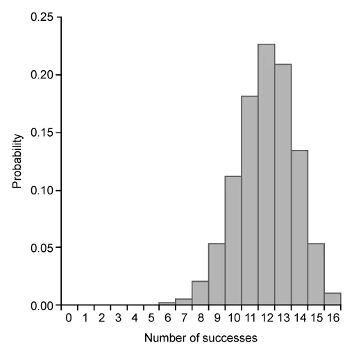
Which of the following graphs represents a binomial probability distribution with parameters n = 16 and p = 0.50 ?
A.  |
|
B. 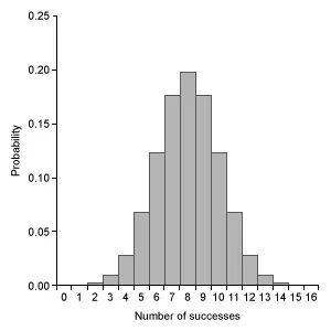 |
|
C. 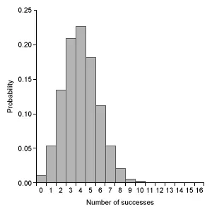 |
|
D. |
|
E. 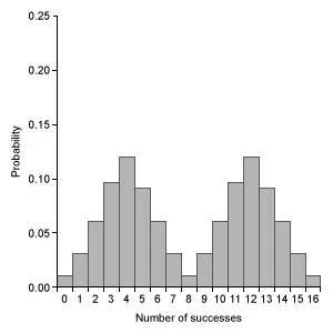 |
Hint:
Consider the mean and standard deviation of the binomial distribution: μx = np and .
Explanation
A binomial probability distribution models the probability of the number of successes of a binomial random variable that meets the conditions of a binomial setting (BINS).
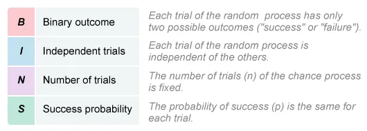
When the parameters of a binomial distribution meet certain conditions, the normal distribution can approximate a binomial distribution.
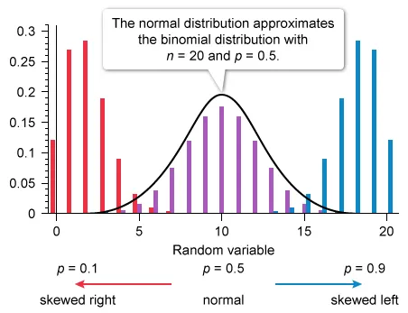
Eliminate Choice A because a binomial distribution with probability of success p = 0.5 is approximated by a normal distribution. Eliminate Choice E because binomial distributions cannot be bimodal.
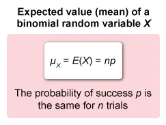
Notice that the remaining graphs each have a different center, so calculate the mean μx of a binomial distribution with n = 16 and p = 0.5 (μx = np).
| μx = np | Mean of binomial variable X |
| μx = 16 × 0.50 | Plug in values |
| μx = 8 | Simplify |
The mean μx of the given distribution is 8. The graph in Choice B is the only distribution with a single peak at 8.
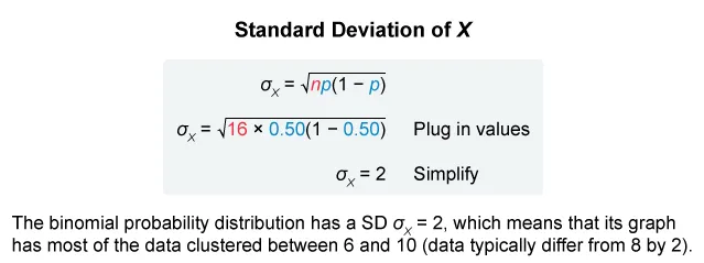
Note: It is also possible to calculate the standard deviation of the distribution to help identify the correct graph.
(Choices A and E) The binomial distribution with n = 16 and p = 0.50 is approximated by a normal distribution, but Choice A is a geometric distribution and Choice E is bimodal.
(Choice C) This graph is slightly skewed to the right and centered at 4, but the graph of a binomial distribution with n = 16 and p = 0.50 is approximately normal and centered at 8.
(Choice D) This graph is slightly skewed to the left and centered at 12, but the graph of a binomial distribution with n = 16 and p = 0.50 is approximately normal and centered at 8.
Things to remember:
- The binomial distribution with parameters n and p has mean (expected value) μx = np and standard deviation
- When p = 0.5, the binomial distribution is approximated by the normal distribution.
Question
A cereal company launches a superhero promotion and decides to include 1 of 5 different superhero figurines in each box of their kids' cereal. The company states that each of the 5 figurines is equally likely to appear in any box of cereal. A statistics student decides to run a simulation to investigate how many boxes of cereal it would take to collect all of the figurines. One trial of the simulation is described by the following steps.
Step 1: Label 5 different tokens 1 through 5 and assign each number to represent a different figurine.
Step 2: Randomly select 1 token at a time with replacement until the 5 different numbers are collected.
Step 3: Record the number of tokens necessary to collect the 5 different tokens.
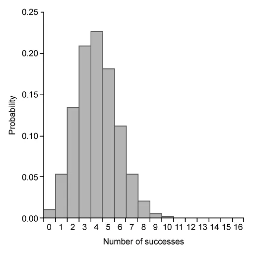
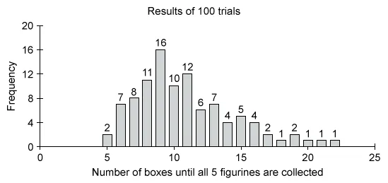
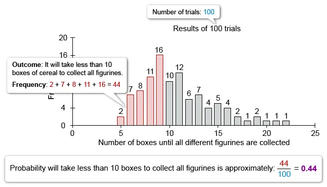
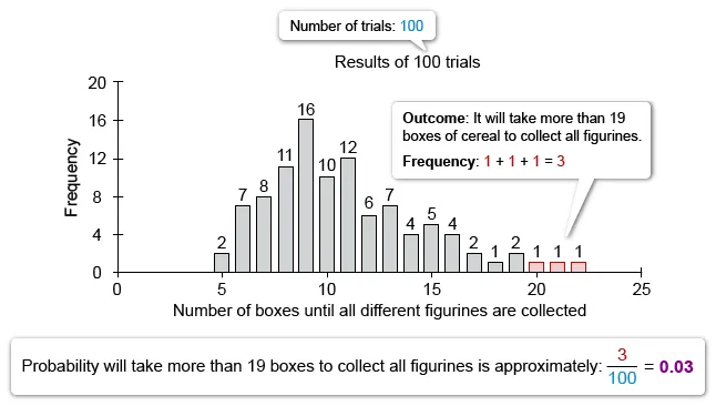
The results of 100 trials of the simulation are shown in the following histogram.
Based on the results of the simulation, which of the following statements is true?
| A. The simulation suggests that the approximate probability that it will take exactly 5 boxes of cereal to collect all 5 figurines is greater than the probability that it will take more than 20 boxes of cereal. | |
| B. The simulation suggests that the probability that it will take less than 10 boxes of cereal to collect all 5 figurines is about 0.55. | |
| C. The simulation suggests that it will take more than 18 boxes of cereal to collect all 5 figurines approximately 5% of the time. | |
| D. The simulation suggests that it will take more than 19 boxes of cereal to collect all 5 figurines approximately 95% of the time. | |
| E. The simulation suggests that it will take at least 22 boxes of cereal to collect all 5 figurines. |
Hint:
To find the relative frequency of a particular outcome in a simulated random process, identify the frequency (count) of the outcome of interest and divide that value by the total number of trials in the simulation.
Explanation
Simulation is the repetition of a random process that closely matches a real-world random event. In a simulation, the relative frequency of each outcome in a random process approximates its probability.
To find the relative frequency of a particular outcome in a simulated random process, identify the frequency (count) of the outcome of interest and divide by the total number of trials in the simulation (ex. 100).
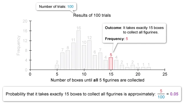
Use the given simulation to analyze each answer choice and determine which statement is true. Notice that it takes more than 18 (19 or more) boxes of cereal to collect 5 different figurines in 5 out of 100 trials.

Therefore, the statement that is true is:
| The simulation suggests that it will take more than 18 boxes of cereal to collect all 5 figurines approximately 5% of the time. |
(Choice A) The approximate probability that it will take exactly 5 boxes to collect all 5 figurines is 0.02, which is equal to (not greater than) the approximate probability that it will take more than 20 boxes (also 0.02).
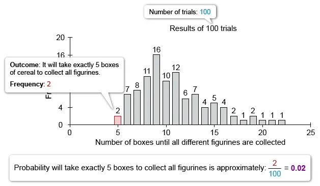
(Choice B) Based on the simulation, the probability that it will take less than 10 boxes to collect all 5 figurines is 0.44, not 0.55.
(Choice D) Based on the simulation, the probability that it will take more than 19 (20 or more) boxes to collect all 5 figurines is 3%, not 95%.
(Choice E) The simulation includes trials where the number of boxes required to collect all 5 figurines was less than 22, so it does not suggest that there must be at least 22 boxes of cereal to collect all 5 figurines.
Things to remember:
- Simulation is the repetition of a random process that closely matches a real-world random event. In a simulation, the relative frequency of each outcome approximates its probability.
- The relative frequency of a particular outcome in a simulated random process is equal to its frequency (count) divided by the total number of trials in the simulation.
Sampling Distributions Practice Test
Question
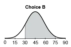
Let X be a normally distributed random variable with mean 45 and SD 15. Which of the following shaded areas represents P(30 < X < 75)?
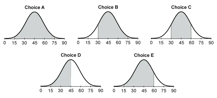
| A. A | |
| B. B | |
| C. C | |
| D.D | |
| E. E |
Explanation
The shaded area should extend from X = 30 to X = 75.
Question
The 1983 Atlantic hurricane season was the least active Atlantic hurricane season since 1930. The season included only four named storms. The named storms as well as their peak wind speeds are given in the following table.
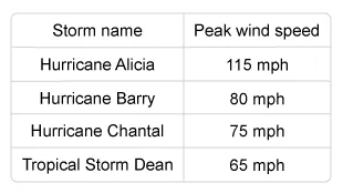
Suppose that a random sample of two storms is selected (without replacement). Which of the following is the probability distribution of the minimum peak wind speed of the sample?
A.  |
|
B. 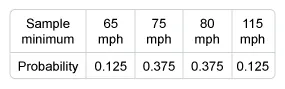
|
|
C. 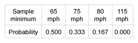 |
|
D. 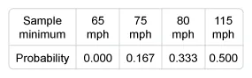 |
|
E.  |
Explanation
There are 12 different samples consisting of two storms selected without replacement. Of those 12 samples:
- 6 have a minimum peak wind of 65 mph (P(Minimum = 65 mph) = 0.500),
- 4 have a minimum peak wind of 75 mph (P(Minimum = 75 mph) = 0.333),
- 2 have a minimum peak wind of 80 mph (P(Minimum = 80 mph) = 0.167), and
- 0 have a minimum peak wind of 115 mph (P(Minimum = 115 mph) = 0.000).
Therefore, the probability distribution of the minimum peak wind speed of the sample is:

Inference for Categorical Data Practice Test
Question
A researcher found that a large-sample 95 percent confidence interval for the proportion of subscriptions that are not canceled before the end of a free trial period is (0.056, 0.124). What is the point estimate for the proportion of subscriptions that are not canceled before the end of the free trial period from which this interval was constructed?
| A. 0.034 | |
| B. 0.068 | |
| C. 0.090 | |
| D. 0.180 | |
| E. It cannot be determined from the information given. |
Hint:
A confidence interval has the general form: point estimate ± margin of error.
Explanation
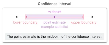
A confidence interval (CI) adds and subtracts a margin of error from a point estimate (sample statistic), so the point estimate is the midpoint of the interval.
It is given that the CI is (0.056, 0.124), so the point estimate must be the midpoint value between 0.056 and 0.124. Eliminate Choices A and D because those values are either below 0.056 or above 0.124.
The midpoint of an interval is equal to the sum of its endpoints divided by 2. To find the midpoint of the given interval, add the lower boundary (0.056) to the upper boundary (0.124) and then divide by 2.

Therefore, the point estimate for the proportion of subscriptions that are not canceled before the end of the free trial period from which this interval was constructed is 0.090.
Note: Point estimates are always at the center of the confidence interval (except in rare cases that will not appear on the exam).
(Choices A and B) These choices may result from mistakenly subtracting the lower boundary from the upper boundary, but it is necessary to add them together and then divide that result by 2.
(Choice D) 0.180 may result from not dividing the sum of the lower and upper boundaries by 2.
(Choice E) This choice may result from a misconception about how an interval is constructed. The point estimate is always contained in the interval constructed from the same sample data.
Things to remember:
A confidence interval adds and subtracts a margin of error from a point estimate (sample statistic), so the point estimate is the midpoint of the interval (except for rare cases that do not appear on the AP exam).
Question
A marketing firm is asked to estimate the proportion of homes in a city with landline phones. A random sample of 150 adult residents were surveyed to determine whether they have a landline phone in their home. Of the people surveyed, 35 percent responded that they have a landline phone. The firm decides to construct a 99 percent confidence interval to estimate the true proportion of homes in the city with landline phones. Assuming all conditions for inference are met, which of the following is closest to the critical value for the 99 percent confidence interval?
| A. 1.645 | |
| B. 1.960 | |
| C. 2.326 | |
| D.2.576 | |
| E. 2.609 |
Hint:
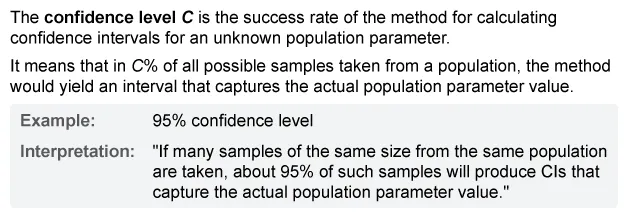
A critical value is a boundary used to identify the middle C% of a probability distribution, where C% is the confidence level of a confidence interval.
Explanation
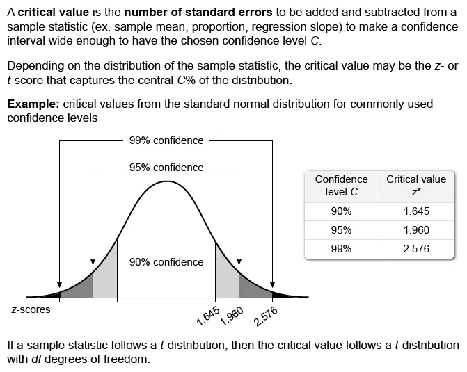
A critical value is a boundary used to identify the middle C% of a probability distribution, where C% is the level of confidence of a confidence interval (CI). It is the multiplier that makes a CI wide enough to have C% confidence.
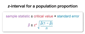
A marketing firm will construct a CI to estimate the true proportion p of city homes with landlines. When conditions for inference are met, the CI for a proportion is a z-interval, and the critical value is a z-score (z*).
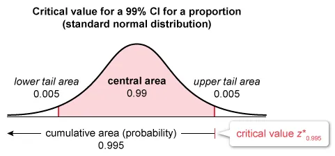
The critical value z* of a 99% CI for p is the z-score that captures the central 99% (and accumulates 99.5%) of the area under the standard normal distribution (z-distribution). The notation for the critical value z* is z0.995.
| To find z0.995, first locate the inverse normal distribution (invNorm) function on a calculator. Input the area under the curve for a 99% CI (cumulative area = 0.995), the mean (0) and standard deviation (1) of the standard normal distribution, and then specify the required tail area (left). |
The answer choice closest to the critical value for the 99% CI for the proportion of adults living in the city who have landline phones is z* = 2.576.
Note: It is possible to determine the critical z-score (z*) with the normal distribution table (see table).
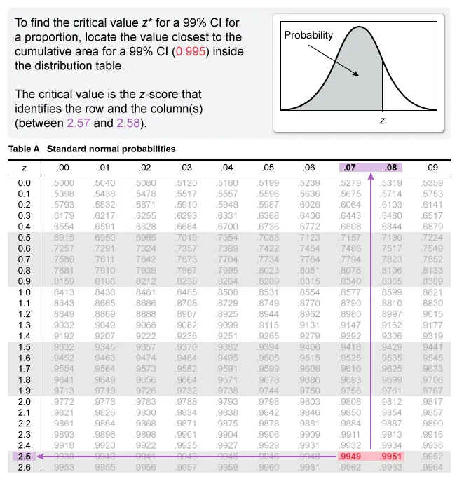
(Choice A) 1.645 results from mistakenly determining the critical value for a 90% CI (z0.95 = 1.645) instead of the critical value for a 99% CI (z0.995 = 2.576).
(Choice B) 1.960 results from mistakenly determining the critical value for a 95% CI (z0.975 = 1.960) instead of the critical value for a 99% CI (z0.995 = 2.576).
(Choice C) 2.326 results from mistakenly determining the critical value for a 98% CI (z0.99 = 2.326) instead of the critical value for a 99% CI (z0.995 = 2.576).
(Choice E) 2.609 results from mistakenly determining the critical value of the CI based on t-distribution with 150 − 1 = 149 degrees of freedom (t149, 0.995 = 2.609) rather than the normal distribution (z0.995 = 2.576).
Things to remember:
- Use a z-interval to construct a confidence interval (CI) for a population proportion p when the conditions for inference are met.
- The critical value z* for a C% CI for p is the z-score that captures the central C% of the area under the standard normal distribution.
Question
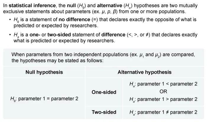
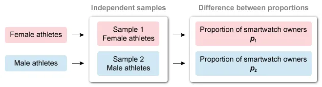
Researchers conducted a survey of 210 randomly selected female professional athletes and 290 randomly selected male professional athletes in a large city. The athletes were asked whether they owned a fitness smartwatch. A total of 180 female athletes and 261 male athletes reported owning a fitness smartwatch. An appropriate hypothesis test was conducted to investigate whether there was a difference between female and male professional athletes in their ownership of a fitness smartwatch. Assuming that conditions for inference are met, is there convincing statistical evidence of a difference between the two population proportions at the significance level of 0.05 ?
| A. No, because the probability of observing a difference at least as large as the sample difference, if the two population proportions are the same, is greater than 0.05. | |
| B. No, because the probability of observing a difference at least as large as the sample difference is less than 0.05. | |
| C. Yes, because the probability of observing a difference at least as large as the sample difference, if the two population proportions are the same, is less than 0.05. | |
| D. Yes, because the probability of observing a difference at least as large as the sample difference is greater than 0.05. | |
| E. Yes, because the sample proportions are different. |
Hint:
Identify the appropriate test and hypotheses, then conduct the test and compare its p-value to the given significance level α to evaluate the statistical evidence.
Explanation
To draw a conclusion about the given data, first identify the appropriate test and hypotheses. Then conduct the test and compare its p-value to the given significance level α.
Researchers selected two independent random samples (female and male athletes) to determine whether there is a difference in the proportion of smartwatch owners between the populations.
The appropriate hypothesis test must evaluate whether there is a difference between two population proportions, so the hypotheses are:
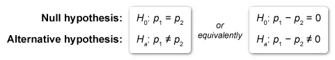
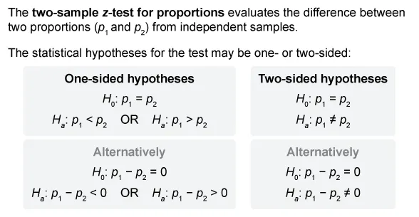
When conditions for inference are met, the hypothesis test that determines whether there is a difference between proportions from two independent samples is the two-sample z-test for proportions.
Notice that Ha is two-sided, so conduct a two-sided, two-sample z-test for proportions and calculate its p-value. Then compare the p-value to the significance level α.
| Locate the two-sample z-test for proportions (2-PropZTest) command on a calculator. Input the given values of the sample statistics for each sample (x1 = 180, n1 = 210, x2 = 261, and n2 = 290), and select the two-sided alternate hypothesis, Ha: p1 ≠ p2. |
If the p-value ≤ α, there is convincing evidence that Ha is true (difference between proportions).
If the p-value > α, there is not convincing evidence that Ha is true (no difference between proportions).
The p-value is 0.143, which is greater than 0.05 (the given significance level α), so there is not convincing evidence in favor of Ha.
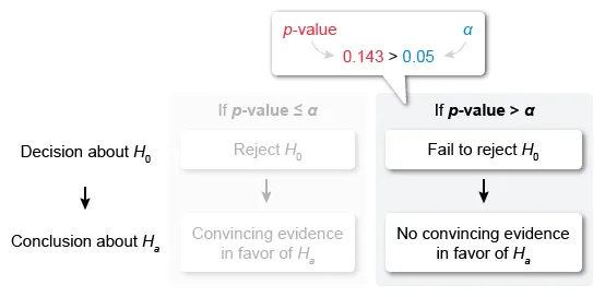
The p-value assumes H0 is true, so the p-value for the two-sample z-test for proportions assumes that the two population proportions are the same.
| Therefore, there is not convincing evidence because the probability of observing a difference at least as large as the sample difference, if the two population proportions are the same, is greater than 0.05. |
(Choices B, C, and D) The p-value is greater than (not less than) the given significance level (0.05), so there is no convincing statistical evidence to conclude that there is a difference between the population proportions.
(Choice E) An apparent difference between two sample proportions does not provide convincing statistical evidence of a difference. It is necessary to conduct a hypothesis test to evaluate the statistical evidence.
Things to remember:
- A two-sample z-test for the difference of proportions compares proportions of two independent samples.
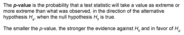
- The p-value is the probability of finding the observed or more extreme results when the null hypothesis H0 is true. The definition of "extreme" depends on the direction specified by the alternative hypothesis Ha.
- To determine whether there is convincing statistical evidence against a null hypothesis H0 and in favor of an alternative hypothesis Ha, compare the p-value to the significance level α.
- If p-value ≤ α, there is convincing evidence in favor of Ha.
- If p-value > α, there is not convincing evidence in favor of Ha.
Inference for Quantitative Data: Means Practice Test
Question
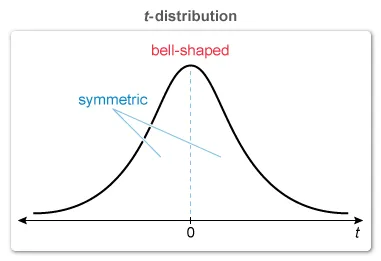
Which of the following statements is true about the t-distribution?
- It is symmetric.
- It is more spread out than the standard normal distribution.
- As the degrees of freedom get smaller, its dispersion gets smaller.
| A. I only | |
| B. II only | |
| C. III only | |
| D. I and II only | |
| E. I, II, and III |
Hint:
The t-distribution is a continuous probability distribution similar to the standard normal distribution. Its spread depends on the degrees of freedom, which is defined differently for different hypothesis tests.
Explanation
A t-distribution is a continuous probability distribution that is similar in many aspects to the standard normal distribution: bell-shaped and symmetric. Statement I is true.
The spread of the t-distribution depends on the degrees of freedom (df), the value of which is defined differently for different hypothesis tests.
An increase in df makes the t-distribution less spread out and closer to the standard normal distribution. A decrease in df makes the t-distribution more spread out and farther from the standard normal distribution.
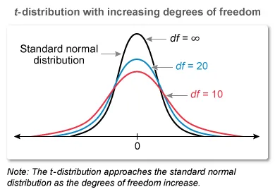
The t-distribution is always more spread out than the normal distribution, and its dispersion gets larger (not smaller) as the degrees of freedom get smaller. Statement II is true, but Statement III is false.
Therefore, of the given statements, only I and II are true.
Things to remember:
A t-distribution is a continuous probability distribution, and (similar to the standard normal distribution) it is bell-shaped and symmetric. The spread of the t-distribution depends on the degrees of freedom (df):
An increase in df makes the t-distribution less spread out and closer to the normal distribution.
A decrease in df makes the t-distribution more spread out and farther from the normal distribution.
Question
A doctor conducted a small study to investigate fasting blood sugar levels in adult patients with diabetes. A random sample of 20 people was selected from the names of all his patients who have diabetes. Of the people in the sample, the mean fasting blood sugar level was 182.23 milligrams per deciliter (mg/dL) with a standard deviation 12.67 mg/dL. The doctor decided to construct a 90 percent confidence interval for the mean fasting blood sugar level, in mg/dL, of all his patients with diabetes. Assuming all conditions for inference are met, which of the following is closest to the critical value for the 90 percent confidence interval?
| A. 1.282 | |
| B. 1.327 | |
| C. 1.645 | |
| D.1.729 | |
| E. 1.960 |
Hint:
A critical value is a boundary used to identify the middle C% of a probability distribution, where C% is the confidence level of a confidence interval.
Explanation
A critical value is a boundary used to identify the middle C% of a probability distribution, where C% is the level of confidence of a confidence interval (CI). It is the multiplier that makes a CI wide enough to have C% confidence.
The doctor will construct a CI for a population mean μ (mean fasting blood glucose level of all his patients with diabetes). The critical value for a CI for μ depends on the method used to construct the CI.

No information is given about the population, so assume that the population SD is unknown. The proper method to construct the CI is a t-interval, and the critical value is a t-score (t*).
The critical value t* of a 90% CI for μ is the t-score that captures the central 90% (and accumulates 95%) of the area under the t-distribution with degrees of freedom (df) equal to the sample size n minus one: n − 1.
It is given that a random sample of 20 people was selected, so the critical value t* is the t-score that accumulates 95% of the area under the t-distribution with 20 − 1 = 19 df. The notation for the critical value t* is t19, 0.95.
| To find t19, 0.95, first locate the inverse t-distribution (invt) function on a calculator. Input the area under the curve for a 90% CI (cumulative area = 0.95) and df = 19. |
The answer choice closest to the critical value for the 99% CI for the proportion of adults living in the city who have landline phones is z* = 2.576.
The answer choice that is closest to the critical value for the 90% CI for the mean fasting blood glucose level of all the doctor's patients with diabetes is t* = 1.729.
Note: It is possible to determine the critical t-score (t*) using a t-distribution table (see table).
(Choice A) This choice results from the error described in Choice C and from mistakenly determining the critical value for an 80% CI (1.282).
(Choice B) This choice results from mistakenly determining the critical value for an 80% CI (t19, 0.90 = 1.327) instead of the critical value for a 90% CI (t19, 0.95 = 1.729).
(Choice C) This choice results from mistakenly finding the critical value for a z-interval (based on the standard normal distribution), but the appropriate interval is a t-interval because the population SD is unknown.
(Choice E) This choice results from the error described in Choice C and from mistakenly determining the critical value for a 95% CI (1.960).
Things to remember:
- Use a t-interval to construct a confidence interval (CI) for a mean μ when the conditions for inference are met and standard deviation (SD) of the population is unknown.
- he critical value t* for a C% CI for μ is the t-score that captures the central C% of the area under the t-distribution with degrees of freedom (df) equal to n − 1.
Question
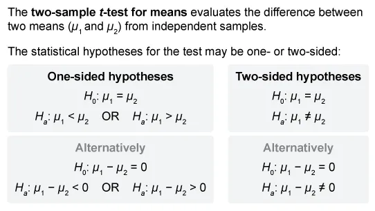
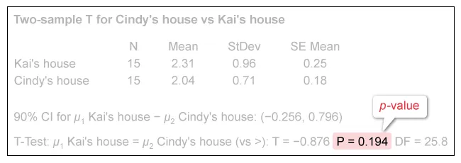
Jane and Ryan are best friends. They live in different cities and take a train whenever they visit each other. Jane believes that it takes her longer to get to Ryan than it does for Ryan to get to her. Jane and Ryan decided to collect data to see if her train transit time is longer than his. They recorded the transit time in hours. After convincing themselves that the assumptions were reasonable, they conducted a two-sample t-test and obtained the following results.
| Two-sample T for Jane's transit time vs Ryan's transit time | ||||
| N | Mean | StDev | SE Mean | |
| Jane's transit time | 15 | 2.31 | 0.96 | 0.25 |
| Ryan's transit time | 15 | 2.04 | 0.71 | 0.18 |
| 90% CI for μ1 Jane's transit time − μ2 Ryan's transit time: (−0.256, 0.796) | ||||
| T-Test: μ1 Jane's transit time = μ2 Ryan's transit time (vs >): T = 0.876, P = 0.194, DF = 25.8 | ||||
Using a significance level of 0.10, which of the following statements best describes the conclusion that can be drawn from these data?
| A. There is convincing evidence that the mean transit time for Jane is greater than the mean transit time for Ryan. | |
| B. There is not convincing evidence that the mean transit time for Jane is greater than the mean transit time for Ryan. | |
| C. There is convincing evidence to conclude that there is a difference in the mean transit time between Jane and Ryan. | |
| D. There is not convincing evidence to conclude that there is a difference in the mean transit time between Jane and Ryan. | |
| E. The t-test cannot be used for samples that are this small. |
Hint:
Use the p-value to determine the statistical significance of the appropriate hypothesis test.
Explanation
To draw conclusions about the given data, first identify the null H0 and alternative Ha hypotheses. Then compare the p-value to the significance level α to determine if there is convincing evidence in favor of Ha.
It is given that a two-sample t-test was conducted to determine whether the mean transit time for Jane (µ1) is greater than the mean transit time for Ryan (µ2), so H0 and Ha are the following:

If p-value ≤ α, there is convincing evidence that Ha is true (mean transit time is greater for Jane than for Ryan).
If p-value > α, there is not convincing evidence that Ha is true (mean transit time is not greater for Jane than for Ryan).
Notice that the given p-value is greater than the significance level α (0.194 > 0.10), so there is not convincing evidence in favor of Ha.

Therefore, the most appropriate conclusion that can be drawn from the data is:
| There is not convincing evidence that the mean transit time for Jane is greater than the mean transit time for Ryan. |
(Choice A) The p-value is greater than the significance level α, so there is not convincing statistical evidence in favor of Ha.
(Choices C and D) These choices describe conclusions based on a two-sided hypothesis test, which evaluates if there is a difference between two means. However, the question asks for a one-sided test, which evaluates if one mean is greater than another.
(Choice E) The sample size is sufficient to conduct the test because the question states that the assumptions were reasonable to conduct the test.
Things to remember:
To determine whether there is convincing statistical evidence against a null hypothesis H0 and in favor of an alternative hypothesis Ha, compare the p-value to the significance level α.
- If p-value ≤ α, there is convincing evidence in favor of Ha.
- If p-value > α, there is not convincing evidence in favor of Ha.
Inference for Categorical Data: Chi-Square Practice Test
Question
A national research group conducted an internet survey in which random samples of 2,000 people who own their home and 2,000 people who rent their home were asked what characteristic of their current living arrangements they consider to be the most desirable. The results of the survey are summarized in the table below.
| Characteristic | |||||
|---|---|---|---|---|---|
| Monthly Costs | Location | Property Features | Size of Living Area | Other | |
| Homeowner | 1,100 | 520 | 195 | 75 | 110 |
| Renter | 950 | 798 | 135 | 45 | 72 |
What is the contribution to the chi-square statistic for homeowners who answered that the size of the living area was the most desirable characteristic?
| A. 0.25 | |
| B. 3 | |
| C. 3.75 | |
| D. 60 | |
| E. 75 |
Hint:
The chi-square statistic is for the chi-square test for homogeneity of proportions.
Explanation
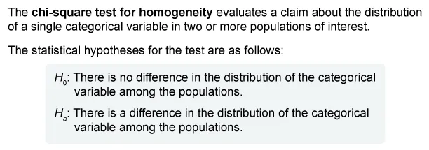
The appropriate hypothesis test to compare the distribution of a categorical variable (characteristic) in two or more populations (homeowners and renters) is the chi-square test for homogeneity of proportions.
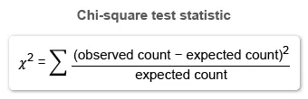
When the conditions for inference are met, use the following formula to calculate a chi-square test statistic (χ²) for the chi-square test of homogeneity.
The individual contribution of a cell is . To determine the contribution of homeowners who answered that the size of the living area was the most desirable characteristic, calculate the observed and expected counts.
Identify the observed cell count of homeowners who said that the size of living area was the most desirable characteristic (75) from the table. Now use the following formula to calculate the expected cell count:
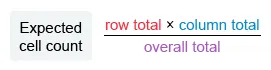
It is given that the overall total is 4,000 (2,000 homeowners and 2,000 renters). Use the table to determine that the row total for homeowners is 2,000 and the column total for characteristic is 120 (calculation).
| Expected Cell Count | |
| Plug in row total = 2,000, column total = 120, and overall total = 4,000 | |
| 60 | Simplify |
Plug the expected count (60) and the observed count (75) into the chi-square statistic formula.
| Contribution to chi-square statistic | |
| Plug in observed cell count = 75 and expected cell count = 60 | |
| 3.75 | Simplify |
Therefore, the contribution to the chi-square statistic for homeowners who answered that the size of the living area was the most desirable characteristic is 3.75.
(Choice A) 0.25 results from mistakenly using (Observed Count − Expected Count) as the numerator of the formula for the contribution the chi-square statistic, rather than (Observed Count − Expected Count)².
(Choice B) 3 results from mistakenly using the observed count rather than the expected count as the denominator of the formula for the contribution of the chi-square statistic.
(Choices D and E) 60 and 75 are the expected count and observed count of homeowners who answered that the size of the living area was the most desirable characteristic.
Things to remember:
- The appropriate hypothesis test to compare the distribution of a categorical variable (characteristic) in two or more populations is the chi-square test for homogeneity of proportions.
- The individual contribution of a cell to the chi-square statistic is .
Question
Consider again the survey of road conditions. For that survey, the researcher conducted an email-based survey of residents living in a large city in the northern U.S. The residents were asked in which region of the city they lived and how they would rate the roads in the city.
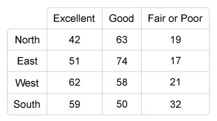
If the researcher instead selected separate random samples of 125 residents living in each region to rate the roads, which of the following procedures would be most appropriate to use for determining if the distribution of road ratings differs among the regions?
| A. Chi-square goodness-of-fit test | |
| B. Chi-square test of independence | |
| C. Chi-square test of homogeneity |
Explanation
It is given that the researcher selected separate random samples of 125 residents living in each region to rate the roads (a stratified sample). The test that compares the distribution of a categorical variable (how residents rate the roads) across different populations (city regions) is the chi-square test of homogeneity.
Question
A researcher conducted an email-based survey of residents living in a large city in the northern U.S. The residents were asked in which region of the city they lived and how they would rate the roads in the city.
Which of the following procedures would be most appropriate to use for determining whether there is a relationship between where people live and how they rate the roads?
| A. Chi-square goodness-of-fit test | |
| B. Chi-square test of independence | |
| C. Chi-square test of homogeneity |
Explanation
It is given that a single sample of residents living in a large city in the northern U.S. was selected and each resident was categorized based on the region of the city in which they lived and how they would rate the roads in the city. The test that evaluates the relationship between two categorical variables (city regions and how residents rate the roads) is the chi-square test of independence.
Inference for Quantitative Data: Slopes Practice Test
Question
The Department of Education of a particular state conducted a study of high school students by selecting 100 random samples, each consisting of 50 high school students. The grade point averages (GPAs) for Precalculus and total SAT scores in each sample were recorded. A 90 percent confidence interval for the slope of the linear regression line between Precalculus GPA and total SAT scores for all high school students was created for each sample. Which of the following is true about the confidence level?
| A. It is expected that about 10 of the 100 confidence intervals will not contain the sample slope of the linear regression line. | |
| B. It is expected that about 90 of the 100 confidence intervals will be identical because they were constructed from samples of the same size from the same population. | |
| C. It is expected that about 90 of the 100 confidence intervals will contain the slope of the linear regression line for all high school students in the state. | |
| D. The probability is 0.90 that 100 confidence intervals will yield the same information about the sample linear regression line. | |
| E. There is 90% confidence that the point estimate of the slope of the linear regression line is correct for each sample. |
Hint:
The C% confidence level represents the confidence with which an interval includes the true population parameter (ex. population slope).
Explanation
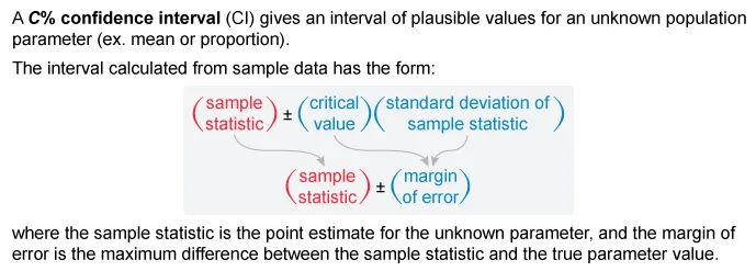
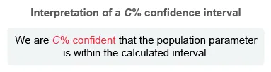
A C% confidence interval (CI) is a range of plausible values calculated from sample data that captures the true population parameter's value with a C% confidence level.
The C% confidence level refers to the percentage of samples of the same size that are expected to result in a CI that includes the true population parameter (ex. slope of the linear regression).

Of the choices, only Choice C defines the confidence level as the percentage of CIs expected to contain the population parameter value. Therefore, the following statement is the best interpretation:
| It is expected that about 90 of the 100 confidence intervals will contain the slope of the linear regression line for all high school students in the state. |
(Choice A) CIs are constructed around a sample statistic (ex. slope), so all CIs will contain the sample slope of the linear regression line.
(Choice B) The confidence level refers to a percentage of CIs expected to contain the population slope, not to the percentage of intervals that will be identical. Samples of the same size from the same population result in different sample statistics (ex. slope), so the intervals are unlikely to be identical.
(Choice D) The confidence level refers to a percentage of CIs expected to contain a population parameter (population slope), not the probability that the sample statistic (sample slope) is correct.
(Choice E) The confidence level refers to a percentage of CIs expected to contain the population slope, not the probability that a certain number of CIs will yield a specific set of values. The probability that a single CI will contain the true population parameter is either 0% or 100%.
Things to remember:
- A C% confidence interval (CI) is a range of plausible values calculated from sample data that captures the true value of a population parameter with a C% confidence level.
- The C% confidence level refers to the percentage of samples of the same size that are expected to result in a CI that includes the true population parameter (ex. population slope).
Question
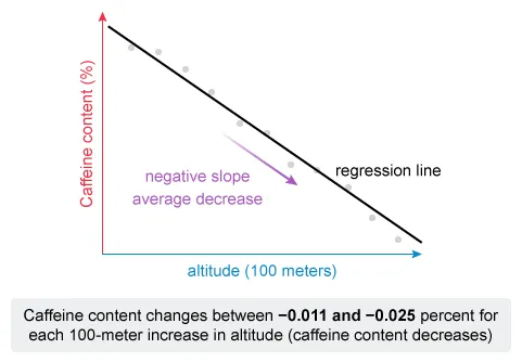
A molecular biologist is interested in the relationship between the caffeine content of green coffee beans and the altitude at which the beans are grown. The biologist collected data on the altitude (in hundreds of meters) and average caffeine content (%) from a random sample of 40 green coffee bean batches in a certain region. A 95 percent confidence interval for the slope of the linear regression line of caffeine content on altitude is determined to be (−0.025, −0.011). Which of the following is a correct interpretation of the interval?
| A. We are confident that the probability is 0.95 that a different sample of 40 green coffee bean batches will result in an increase, on average, of caffeine content between 0.011 and 0.025 percent for each 100-meter increase in altitude. | |
| B. We are confident that the probability is 0.95 that caffeine content will decrease, on average, between 0.011 and 0.025 percent for each 100-meter increase in altitude. | |
| C. We are 95% confident that, for any sample of green coffee bean batches, the caffeine content will decrease, on average, between 0.011 and 0.025 percent for each 100-meter increase in altitude. | |
| D. We are 95% confident that the caffeine content increases, on average, between 0.011 and 0.025 percent for each 100-meter increase in altitude. | |
| E. We are 95% confident that the caffeine content decreases, on average, between 0.011 and 0.025 percent for each 100-meter increase in altitude. |
Hint:
A confidence interval is an interval of plausible values that, with a specific level of confidence, should contain the unknown value of a population parameter.
Explanation
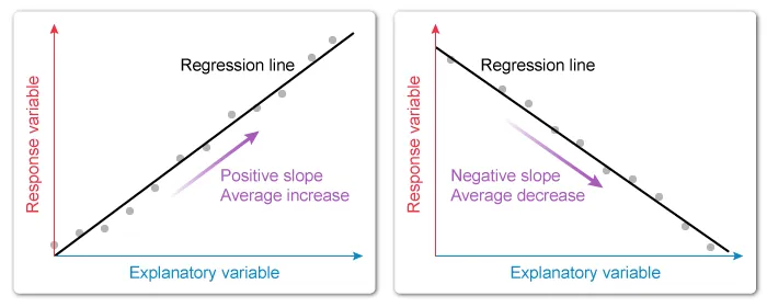
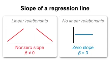
The slope of a regression line is the average change in the response variable per unit increase in the explanatory variable.
A positive slope represents an average increase in the response variable as the explanatory variable increases.
A negative slope represents an average decrease in the response variable as the explanatory variable increases.
It is given that a molecular biologist conducted a regression analysis of caffeine content on altitude, so caffeine content is the response variable and altitude is the explanatory variable.
Notice that the given interval (−0.025, −0.011) for the slope of the regression line contains only negative values, so caffeine content decreases (on average) as altitude increases. Eliminate Choices A and D.
Now consider the definition of a confidence interval (CI).
Therefore, the correct interpretation of the interval is that we are 95% confident that the caffeine content decreases, on average, between 0.011 and 0.025 percent for each 100-meter increase in altitude.
(Choices A and D) The given CI (−0.025, −0.011) contains only negative values, so the caffeine content is expected to decrease (rather than increase) on average as altitude increases.
(Choice B) A confidence level does not calculate the probability that the slope of a population regression line is within the CI. The probability that the slope of a population regression line is in the interval is either 0% or 100%.
(Choice C) A CI provides an interval of plausible values for the slope of the population regression line. Each sample may result in a different 95% CI for the slope due to sampling variation.
Things to remember:
- The slope of a regression line is the average change in the response variable per unit increase in the explanatory variable.
- A confidence interval (CI) gives an interval of plausible values that, with a C% level of confidence, should capture the unknown population parameter.
Question
A doctoral-level kinesiology student selected a random sample of female students registered at the campus recreation center and collected data on their cardio fitness score and body mass index (BMI). She wants to calculate a 90 percent confidence interval for the slope of the regression line of cardio fitness score on BMI in the population of female students registered at the campus recreation center. Which of the following statements must be true in this situation to use a t-interval for the slope?
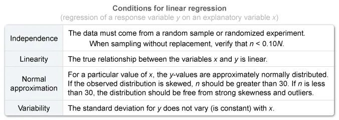
- The variability of cardio fitness scores is the same for all BMI values.
- The mean of the cardio fitness scores is the same for all BMI values.
- The mean of the cardio fitness scores changes at different rates as BMI values increase.
| A. I only | |
| B. II only | |
| C. III only | |
| D. I and II only | |
| E. I and III only |
Hint:
Consider the conditions in which a t-test for the slope is valid (independence, linear relationship, approximately normal distribution of the response, and constant variability of the response).
Explanation
A student will use a t-interval to construct an interval for the slope of the regression line of cardio fitness score (response variable) on body mass index (BMI) (explanatory variable) in the population of female students at the recreation center.
A t-interval to estimate the slope of the population regression line is valid under the following conditions:
Consider each statement and determine which must be true to use a t-interval to estimate a regression slope.
Statement I: The variability of cardio fitness scores is the same for all BMI values.
The t-interval for the slope requires that the variability (standard deviation) of the response variable (cardio fitness score) does not vary with the explanatory variable (BMI).

Statement I must be true to use a t-interval for a slope, so eliminate Choices B and C.
Statement II: The mean of the cardio fitness scores is the same for all BMI values.
For a linear relationship, the mean of the response variable is not constant across the values of the explanatory variable.
If there is no relationship, the mean of the response variable may be constant across the values of the explanatory variable. Statement II does not need to be true, so eliminate Choices B and D.
Note: If the mean of the response variable is constant across the values of the explanatory variable, then the slope is zero (no linear relationship).
Statement III: The mean of the cardio fitness scores changes at different rates as BMI values increase.
The t-interval for the slope requires that the relationship between the response (cardio fitness score) variable and the explanatory variable (BMI) be linear.
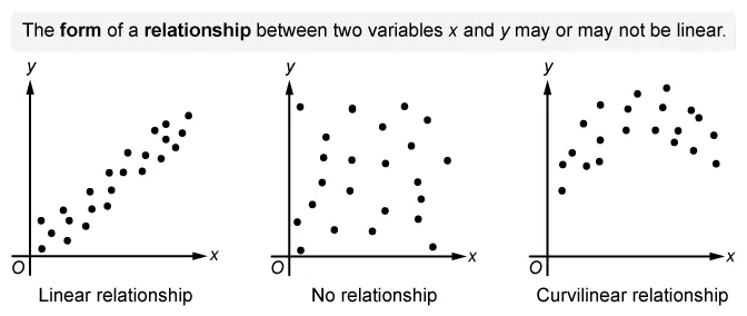
For a linear relationship, an increase in the explanatory variable results in a constant change in the mean of the response variable. Statement III is not true for a linear relationship, so eliminate Choices C and E.
Of the given statements, only Statement I must be true to use a t-interval for the slope in this situation.
|
Things to remember:
- A t-interval for the slope of the regression line estimates the slope of the population regression line.
- The conditions for a t-test for the slope to be valid are independence, linear relationship, approximately normal distribution of the response, and constant variability of the response.


UWorlds multiple choice questions are similar to the ones on the official AP exam and allowed me to time myself for each question. This was very helpful for me as I was able to answer questions faster and could finish the questions on the actual exam. The explanations for each question went in-depth and gave important details pertaining to events in the timeline. Through this, I was able to gain important skills for the exam and get a 5.
See MoreBefore, I had a hard time studying and staying focused because it was just boring, but now with UWorld, not only can I focus, but I actually feel motivated to learn!
The explanations were clear and I could practice the question based on units. I got a 5 in the end!! So, I think it’s very helpful and I’ll be using it to study for my future exams 🙂 You guys provide so many different functions to help students like me, and I really appreciate it, it’s really worth the money.
See More